Profile Value Change After Billing

Profile values play a crucial role in the billing and invoicing process for customers.

Once billing is completed, it is imperative that profile values remain unchanged to maintain the accuracy of calculations. Any alterations to profile values necessitate the reversal of billing procedures followed by rebilling the customer.

This basic configuration to prevent profile value changes post-billing is present within the Profile Allocation screen.

The below demonstration will illustrate this configuration.

Additionally, certain scenarios may arise where billed profile values for specific profiles require modification. In such cases, the Function Activation feature, as outlined in SAP Note 3222145, is made available.

Notably, in the presented example, the billing checkbox for Profile Role 0001 remains unticked. This checkbox serves to validate any alterations to profile values within the billed period, triggering an error message if necessary.

If I try to Change the Profile Values through EEDM01 transaction, we can see that the Profile Values open in Change Mode.

If Now I change the Configuration as shown below, the Profile Values give an error in Change Mode for the Billed Period.

Now with the Configuration in place I have activated the Node in the BRF Application as shown below and we can see that the Profile is now opening in Change Mode.

The BAdI is ISU_EDM_BILL_CHECK.

This was a very short blog on Profile Values. Thank you..

Please note that this post was authored three years ago. However, I recently discovered that although it was marked as published, it was not visible online. Consequently, I have appended new content pertaining to Feature Activation and reissued the publication.

That’s it. Thank you 😊

EDM – Cumulative Profile Values

I have been blogging for a while on niche subjects that may appear minor to some, yet they prove valuable in imparting insights into the complexities and potentials within the SAP Utilities system.

Today I am writing about a small check box available in the Profile Header Screen – Cumulative Values (Technical name – VALUECUM).

The SAP help document states – “Indicates that at time t the value is dependent on the values of times t-n”.

This implies that we can store Cumulative Meter Readings in Profiles. However, Profiles labeled with Cumulative Values cannot be directly utilized in RTP Billing. The answer is negative as per SAP Note 2008164. Before use, these profiles require calculation. The process involves using them as input for a Formula Profile employing the MR_TO_CONS formula. Subsequently, this Formula Profile becomes eligible for utilization in RTP Billing.

Formula – MR_TO_CONS is a successor to the previous Formula – ACCU_TO_BALANCE in S/4HANA (SAP Note – 2594632). Also, this Formula cannot be used in an RTP Interface.  

Now the blog is structured as per below points –

• I have first tried to show a simple Profile with Cumulative Values been used in RTP Billing. It will not give the desired result.
• Formula Profile is created, and Calculations done.
• Formula profile is used for RTP Billing.
• Check if Formula Profile can handle Meter Reading Overruns.

RTP Billing using Profile having Cumulative Profile Values

Below are the Profile Values – In increasing Order.

I will now initiate the billing process, examining the result parameters and presenting the line items in the billing document. As previously indicated (SAP Note – 2008164), RTP Billing lacks the capability to manage Cumulative Profile Values. Instead, it simply aggregates all the consumption, deviating from the expected behavior.

Creating Formula Profile and Calculations

I’ve created a Formula Profile featuring the MR_TO_CONS formula. The input parameter includes the previously utilized profile. I assigned this Formula Profile to the device, replacing the previous allocation. I then initiated the formula calculation to examine the results.

Formula Profile Calculation done.

Using Formula Profile in RTP Billing

Now RTP can bill correctly.

Meter Reading Overruns

Now what will happen if we pass Profile Values which are random, or I should say show Meter Reading Overruns/Rollover as shown below.

When the Formula Profile Calculation runs it shows like this.

From the code above, it’s evident that the logic only checks if the calculated value is below 0, in which case it passes the value as 0. However, it does not verify the presence of Meter Reading Rollover or other issues, contrasting with the Meter Reading Validations performed by the Discrete Meter Reading Process.

That’s it. Thank you 😊

Replacement Value for Operands

A Very short Blog covering a minor topic, but which plays an important role in Tariff Configuration.

We know the Hierarchy of Reading Facts taken by Utilities Billing engine –

• Installation Facts
• Rate Category Facts
• Rate Facts grouped under Fact Group

How is the Rates linked to the Installation –

• The rates are allocated to the Installation indirectly via the allocation of the Rate Types.
• The rates to be used are found in Rate Determination.
• The Rate category is maintained in the Installation time Slice.

Now to the topic in hand – When proposing Operands, we need to select any of the 4 Radio Buttons, in some cases only 3 buttons are in Change mode and in some 2 Buttons.

The default selection is Normal Operand Value, representing the standard configuration for maintaining operand values. When enabled, it mandates the specification of an operand value.

Required Value – This option can be applied within the Rate Category Facts or the Rate Facts. If we assign this replacement value to an operand in the Rate Category Facts, the operand is suggested for maintenance across all installations linked to the allocated Rate and Rate Category. In such cases, it becomes necessary to provide a value for this operand in the Installation Facts unless a value is already entered in the Rate Category Facts.

However, if we define this replacement value for an operand in the Rate Facts and also provide a value for the same operand in the Rate Category Facts, the operand will not be suggested for maintenance in the Installation Facts.

Optional value for operand – This replacement value can be applied in either the rate category facts or the rate facts. If assigned to an operand in the Rate Category facts, the operand is suggested for maintenance in all Installation Facts associated with the allocated rate category. It is mandatory to provide a value for this operand in the Installation Facts if no value is entered in the Rate Category facts.

Operand value determined at Runtime – This replacement value signifies that the billing value for this operand is not calculated until the billing process. It is essential to specify this replacement value if the operand is updated in later rate steps as an output operand for a Rate step.

Required Value Operand Value Analysis

Made the Operand required in the Rate Fact Group as shown below.

Made it required in the Rate Category Facts as shown below.

Now when we see the Installation Facts is shows as below.

Now I shall maintain a value in the Rate Category Facts for this as shown below.

Rate Facts still has the same check box as before.

Now for the Installation we are not getting the Operand to be maintained by default.

If Now I maintain the Rate Facts as Normal Operand Value as below –

And the Rate Category Facts as Required, then the Installation Facts would require the Operand Maintenance.

Optional Value for Operand Analysis

Made it Optional in the Rate Fact Group as shown below.

Made it Optional in the Rate Category Facts too.

Now In the Installation Facts we can see the below.

Now I shall maintain the Rate Category Facts as shown below. Rate Facts will continue with Optional.

Now for the Installation we are not getting the Operand to be maintained by default.

Let’s try a different combination now –

In Rate Fact group Facts, I have selected the Required Value for Operand as shown below

And for Rate Category Facts I have selected the Optional Value for Operand as shown below

Now in the Installation, it shows as below. Therefore, it’s clear that the Facts Status at the Installation level is driven by the Facts Value Status maintained in the Rate Category Facts & is not influenced by the Rate Fact Group Facts.

If I reverse the Operand Value selection i.e., Optional Value in Rate Fact group and Required in Rate Category Facts, we see the below in the Installation.

That’s it for now.. 😊

Changing the Consumption

In certain scenarios, the Meter Reading captured in the field does not align with the expected Consumption. This can occur if the Meter is already known to be faulty, damaged, or inaccessible. In such cases, Standard Estimations or custom estimations can be triggered to obtain an Estimated reading. However, this Estimated reading is calculated by the system. Sometimes, as per the Business Process, the Utility agent may need to modify the Consumption (due to factors like Billing Factor changes) to reflect the real-world situation. In these cases, Standard SAP provides an option for the Utility to adjust the Consumption to be billed after the Meter Reading has been uploaded.

There are two types of Meter Reading: the Reading captured directly from the Meter by the Meter Reader and the Reading used for billing purposes. In these scenarios, we are not modifying the Meter Reading uploaded to SAP by the Meter Reader, but rather adjusting the Meter Reading (specifically the Consumption) that will be billed in SAP.

The field “Consumption” (in this case, 93.33 units) is the focus of discussion. It is calculated at runtime based on the uploaded Meter Reading (MR Recorded). It’s important to note that this field is visible in the system but not available in the API calls for Meter Reading Upload. This means that any changes to the Consumption must be made within the SAP system and cannot be done through the Standard API. In the SAP system, a custom MR Note is required, which, when updated by the Meter Reader, triggers the logic to modify the Consumption or serves as an outlier for the Utility to take action.

In the provided example, the Previous Reading was 100 units, and the system estimated the consumption as 93.33 units. Therefore, the Current Meter Reading is 193.33 units, which is the same as the Meter Reading to be billed. The simulated billing document line item reflects this.

Next, the Consumption was manually changed from 93.33 units to 101 units, and the Meter Reading was saved. It’s important to note that changing the Consumption does not alter the Meter Reading uploaded to SAP. The difference lies in how the Meter Reading uploaded and the modified Consumption are saved in Table EABL and the Consumption used for Billing.

In the updated data, we can see that the consumption has changed to 101 units.

The billing document now considers 101 units for Billing instead of the 93.33 units derived from the Current Meter Reading and Previous Meter Reading.

The Billing View of the Installation includes an additional column showing the difference between the Meter Reading uploaded and the Meter Reading used for Billing. This change is also reflected in Table EABL.

For the next month, estimation was performed again, but the Consumption was not altered. The Estimation logic used the Meter Reading Uploaded as the basis for estimation, as seen in the two columns below.

If the Consumption is modified in EL29, as shown, the difference becomes evident once again.

Entering an excessively high Consumption triggers a standard Validation Error according to the system’s configuration.

That’s it 😊

Ignore Estimated Readings during Extrapolation

This is a small blog post talking about a simple check box in Device Management Configuration.

Trying is to explain how it works.

Below are some Meter Readings with the Move – In done on 1^st Jan 2023 and Periodic Reading done 27^th January (Actual Reading) followed by Periodic Reading on 24^th February (Estimated Reading)

Now as we see below the configuration is unchecked – Ignore Est.

If we select this Checkbox the system only selects Active Meter Readings for Extrapolation.

If we try Estimation for 29^th Match 2023 Billing period, the system is able to find a representative period and estimates from the past period. Here it takes into both the Actual and Estimated Readings.

Number of Days for Representative Period is 31 + 24 = 55 Days

Consumption for Representative Period is 550 units

Billing Period Days is 4 + 29 = 33 Days

Expected Consumption is (550 * 33 / 55) = 330 units.

Now I have selected the Checkbox and let’s see what the System does for different combinations of Meter Reading Type.

Scenario 1 – If I try Estimation for 29^th Match 2023 Billing period after the Checkbox is active , the system is not able to find a representative period and estimates from the Periodic Consumption.

Periodic Consumption maintained in the system – 12 units per Day.

Billing Period Days is 4 + 29 = 33 Days

Expected Consumption is ( 33 * 12 ) = 396 units.

Scenario 2 – Now the Meter Reading for January and February Month is Estimated as shown below.

Now if we try to Estimate for the March Month, as we see that the system is not able to find a representative period and estimates from the Periodic Consumption. Calculation is same as Scenario 1.

Scenario 3 – Now the Meter Reading for January Month is Estimated and February is Actual Meter Reading as shown below.

Now if we try to Estimate for the March Month, as we see that the system is able to find a representative period and estimates from the Past Meter Readings. It takes the Consumption between the two Actual Meter Readings to find the repsentative period and does the Estimated Consumption Calculation.

Number of Days for Representative Period is 31 + 24 = 55 Days

Consumption for Representative Period is 550 units

Billing Period Days is 4 + 29 = 33 Days

Expected Consumption is (550 * 33 / 55) = 330 units.

Summary – If the checkbox – Ignore Est. is checked then the System tries to get a Representative Period between Actual Readings, if not found it uses Periodic Consumption.  

That’s it. 😊

Leading Zeros in Serial numbers

As always, a small post.

This is mainly about a scenario where the Meter Number available in the field have Zeros as a prefix. Now these need to be migrated to SAP with the Zeros as prefix.

We know that Standard SAP applies Conversion Routines on display of Serial Numbers in the GUI.

Like if we check an ISU Equipment through IQ03, the serial number wouldn’t show any leading zeros but the same field through SE16N would show zeros as unconverted value up to the limit of the field length. This also doesn’t fulfil the requirement cause if the Serial Number in Field is 00123456, the unconverted value would be 000000000000123456 and the value shown in GUI is 123456 in SAP. The Requirement is that the Serial Number if given as 00123456 from the Field, should be stored in SAP as 00123456 and displayed as 00123456 in the SAP GUI screen.

The below is shown through an Example.

Gave the Serial Number with Leading Zeros in Transaction IQ01.

The leading zeros have been removed as shown below.

If I check the Table EQUI after saving the device, the Equipment number is converted as shown below. Also, the Serial Number SERNR is converted. We don’t want SERNR to be converted. It should store the Value as 00123457. Remember we are using numeric Values not Alphanumeric Values here.

There are some Notes available which talk about this; therefore, I will directly come to the point.

We need to enable the check through Transaction OLZSN. Table is ADLZSN.

Default is a blank value.

Now for my Serial Number Profile 0001 which is maintained in the Material, I have activated this check. Below screenshots shows that.

Now I am creating a Device with leading zeros as shown below. We can see that Zeros as prefix are not removed.

If I check the Table EQUI after saving the device, the Equipment number is converted as shown below. But the Serial Number SERNR is not converted. It still shows as expected number with leading zeros.

That’s it. 😊

Consumption field in EL31 – Manual Monitoring

This is a small post on EL31 – Manual Monitoring transaction.

There are recent notes talking about this.

2984321 – Interface note: EL31, additional fields in meter reading document hit list – SAP ONE Support Launchpad

2984316 – Activation levels for additional fields in EL31 hit list – SAP ONE Support Launchpad

The problem statement here is that we try to add the Consumption field from the layout, it always displays 0 value.

But if we visit the details screen, then the field shows value in the detail screen.

To correct this behaviour – We need to implement a BADI ISU_MR_MONI_CUSTDAT. For this BADI – method ALV_DETAILVIEW_FIELDS just write this – XY_DETERM_CONSUMP = ‘2’.

Now we can see the Consumption coming in EL31 screen.

Thank you 🙂

Profile Interval Size Change

As always this is a small post.

While creating EDM Profiles we must mandatorily give the Interval Size. By standard in the system – 5min,10 min, 15 min, 30 Min, 60 Min and 1 Day. We can define custom sizes but generally the standard interval size suffices the requirements.

Now this blog is about how the standard SAP system handles EDM Profiles with different interval sizes. I am using a Formula Profile with standard EDM formula MULTI02.

MULTI02 has 2 Input Parameters – Quantity (unit of measurement KWH) and Factor (no unit of measurement). Output is Quantity (Unit of Measurement KWH).

For this demo I have given different Interval Lengths – Formula Profile with 5 mins, Quantity Profile with 15 mins and Factor Profile with 30 mins Interval size.

For Values I have given these values for the whole period – Quantity as 2 KWH and Factor as 3.

Therefore, Quantity Profile with 2 KWH for 15 mins should be 0.67 KWH for 5 Mins and similarly Factor Profile with 3 for 30 mins should be 0.5 , giving the Factor Profile of 5 mins Interval as 0.67*0.5 = 0.34.

I have mentioned only rounded values in the post but in the system it’s in many decimal places. Now when I run the Calculation workbench, I see the calculated Formula Profile Values as below.

It seems the calculation has ignored the Interval size of the Factor Profile here. As 0.67 * 3 gives 2 (round about). Question arises as to why this was done and where can I see the relevant logic. The relevant logic can be seen in Class CL_DEF_IM_ISU_EDM_PROFILE_CONV , in Method CONVERT_DATA. This is part of Note 3073840.

As the above logic shows, depending on the Profile Value Category the Profile Values are manipulated. Profile with Profile Value Category – Power, Price and Factor do not change the Profile Values based on Interval size changes but only Profiles with Profile Value Category – Quantity and Amount, change the Profile Values with Interval size Changes.

Therefore, in the demo shown earlier, the Profile Value for Quant Profile was changed from 2KWH for 15 mins to 0.67 KWH for 5 mins, but the Profile Value for Factor Profile was not changed (from 3 for 30 mins). It remained same for 5 min Interval too.

Same logic applies to the Unit of Measurement, like from KWH to MWH conversion.

Thank you 😊

Convergent Charging – Shared Allowances

This is a small post on Sharing Allowances used in Convergent Charging. Though not a new concept but it’s not used so frequently.

Note – I write these posts as a reminder on how I had worked on it or how I had resolved a particular issue. If details are needed on the objects/processes, links are mentioned. 😊

I would have another post on Sharing Counters later.

All about Allowance can be found here. All about Sharing Allowances can be found here.

There are specific parameters which need to be configured for Shared Allowances which can be found in this note – 2498054.

Now I shall repeat (copy/Paste) some Text on Shared Allowance – just for quick reference.

Shared Allowances can be shared between Provider Contracts that belong to different Subscriber Accounts or same Subscriber Account. When we create Shared Allowances, we assign the same unique identifier to the Shared Allowance or to a group of Shared Allowances i.e., multiple Shared Allowance can also be shared. Provider contracts use this unique identifier to access the Shared Allowances of the group.

Do not get confused with the Unique Identifier each Allowance has with the Shared Allowance Share Identifier. They are different objects as highlighted below.

Now there are different scenarios where Shared Allowance can be used and where Sharing Counters should be used – depending on the object capabilities of course.

Sharing Allowances Between Provider Contracts within a Subscriber Account – An allowance is linked to a Provider Contract, which can be itself linked to a parent Provider Contract. A Provider Contract can access the allowances of its parent Provider Contract but vice versa is not allowed.

Sharing Allowances Between Provider Contracts from Separate Subscriber Accounts – For Shared Allowance, the Provider Contract that owns the allowance specifies a unique share identifier during the creation of the shared allowance. The other Provider Contracts (called “members”) from other Subscriber Accounts, use this share identifier to consume the Shared Allowance.

In the Create Allowance Operator component, the user selects the option if an allowance is to be shared or not. To build up a group of Shared Allowances, one or several provider contracts (owners) can create several Shared Allowances using the same share identifier. To use the Shared Allowances, the member provider contracts must send allowance consumption events through the Allowance Event Sender component that is configured to use the same share identifier. Only Event-Based Trigger components of these shared allowances are activated, and thus their logic are executed.

Definition (Tab) –

We have an important Section – Scope, where we need to Select one of the three options for the action perimeter that suits the business requirements:

• Only Allowances of the Contract.
• Allowances of the Contract and its Parent.
• Only Shared Allowances.

Share Identifier is for identifying the group of shared allowances to which the system sends an allowance event when executing the Allowance Event Sender component at runtime.

Selection (Tab)

Here we can define the conditions for selecting the allowances that will receive the allowance event. The counters that are defined in the allowance interface for shared allowances are not available for selection.

Sorting (Tab)

On the Sorting tab of the Allowance Event Sender component, we can define the sorting criteria based on the two-levels:

1. The first level is ordering the criteria based on their position (rank) in the table. This defines the sending priorities.
2. The second level is defining the ascending/descending order for each criterion.

More on Allowance event Sender Operator can be found here.

Now the basic principle Shared Allowance follows is that it starts deducting the Allowance (which is shared) which is initiated or activated first. Let me give an Example – I have 2 Shared Allowances for SMS – say ALLSMS1(with Provider Contract A) and ALLSMS2(with Provider Contract B) with same unique Share ID. When a SMS usage is sent for Provider Contract A it shall deduct the Allowance (ALLSMS1) for Provider Contract A. Now a SMS usage is sent for Provider Contract B, it should deduct the Allowance for Provider Contract B from ALLSMS2, but it deducts it from ALLSMS1. This happens because Shared Allowance deducts it from the shared bucket which was activated or initiated first in this case ALLSMS1. Once that is exhausted then ALLSMS2 is consumed. This is the standard behaviour as the System pools the Shared Allowances in a bucket and consumes it sequentially if they are of the same usage type.

If we want to ensure that the system should first consume the specific Shared Allowance allocated for the Provider Contract and if exhausted then only consume the Shared Allowance of other Provider Contracts (those with the same Share ID), we need to play around with the Selection Tab in Allowance Event Sender and also how the Allowance Event Sender is called.

We would need to first check with the Provider Contract (for which the Usage was sent) if it has pending Allowances. This can be done by adding a Unique filter in the Selection Tab to first select the Provider Contract. If the Allowance is exhausted, then check for the other Shared Allowance bucket for consumption. This would mean to again call the Allowance Event Sender without that unique filter.

We can also play with the Sorting Tab inputs. Once the call comes to the Shared bucket for the consumption based on the filer applied here, we can mark which Shared Allowance in the bucket should be consumed first. Like I can set a priority in the Provider Contracts whose bucket should be consumed first or based on when the Allowance is expiring.

Thank You ..

Ignore Contract Allocation during Extrapolation

In the past I have blogged on Estimation process that is followed in SAP for Utilities with the Periodic Consumption usage, how Weighing Procedure is leveraged and how the Base Representative period is calculated.

Now Estimation follows many rules, and we get an Estimated value when we click on the ‘Estimate’ button. To check and finally ascertain how the system or I should say algorithm derived that Estimated Consumption is always a task even though we know the steps system takes. 😊

Now, what if we don’t want SAP to estimate any consumption for the Billable register. Generally, the standard followed method is to check Past Meter Readings or if not available or representative use the Periodic Consumption.

The Contract plays an important role here. If, contract is not there in the Installation then the Estimated Consumption is ZERO as an empty Premise cannot consume Energy in an ideal world. If Contract is present the usual estimation follows.

A short demo below –

The Delivery Meter Reading ( Meter Reading Reason is 19 ) as shown below – 0 KWH. This Meter is not installed anywhere currently.

When I click on the Estimate button, the Estimated Meter Reading is 0 KWH.

Below are the details on the Validations.

Now I have updated the Delivery Meter Reading to 10 KWH as shown below.

If I now try to Estimate the Meter Reading it shows zero Consumption.

Remember, the Independent Validations maintained in the Configuration have still not triggered as seen above.

Now I have installed the Device (Full Installation) but the contract is not created i.e. no Move -In.

Now I try to estimate the Meter Reading – It still gives Zero Consumption as without Contract how can there be any consumption. No Independent Validations have been triggered.

Now I have done the Move-In and trying Estimation. Do remember the Delivery Meter Reading is 10 KWH and Periodic Consumption is 1KWH per day.

If I estimate for the next month –

Now if we don’t want SAP to estimate any consumption for the Billable register. There is a checkbox in the Rate Type Configuration titled ‘Ignore the contract allocation of the register during extrapolation’ abbreviated as CA.

This indicator influences the analysis of the contract allocation during extrapolation of registers. If we install a register for billing in an installation and use a rate type for which this indicator is set, the installation is interpreted to have no contract allocation whether a contract exists or not.

Generally during extrapolation of a register, the system checks for which periods a contract is allocated to the corresponding installation. The periods that are not allocated a contract are given an estimated consumption value of zero. This is as mentioned earlier – no energy should have been consumed if no Business Partner is allocated. Therefore, if we set the Ignore Contract Allocation of Registers During Extrapolation indicator, a consumption value of zero may be estimated even though a contract is officially allocated to the installation.

We can set the indicator for rate types that we want to use in installations whose contract allocation does not reveal anything about the consumption behaviour. Such cases can arise for deregulation or for register relationships for example.

Now if we try Estimating the Meter Reading it doesn’t use Past Meter Reading or Periodic Consumption.

The previous screen was showing a Validation Error for Zero Consumption, so I removed it from the configuration. The screenshot again.

That’s it. Have a Good Day !!

Reversal Category for Billing Reversal

As per the Standard Transaction for Billing Reversal or Invoicing Reversal, we need to give the Reversal Reason. These Reversal Reasons have a specific purpose and are configurable. The Reversal Reason Category are actually defined by SAP.

As Reversal Reason is a configuration item, any Reasons mentioned below is subject to change and would be different in any other SAP Utilities system. But the field which stands for Reversal Reason Category is pre-defined by SAP (the values) and can be used in Reporting and drawing inferences(why,when and where).  Now a standard variant IF14 is used which checks on the Reversal Reason Category and can be used as per the applicable reason.

To execute a Simple use Case, I have configured a custom out sort which reads an Installation fact. This Installation fact is updated within the IF14 variant scope to inform the system that this Billing document has to be out sorted, so that it can evaluated again before been Invoiced and sent to the customer. I can also include variants to add new price points or give rebates. All this is possible.

This is the Out sort configuration.

This is the Reversal Reason configuration for Billing Reversal.

Now I have reversed a Billing document giving the Reversal Reason as 00 – Theft of Service and hopefully all the Utility processes for addressing the Theft process is done and now as shown below the Billing process was executed again and the Billing Document was outsorted.

The whole idea of this post is that we have a Reversal Reason Category which can be used to capture relevant data points to process on why a ‘reversal’ was done, whether any corrective steps have been taken into consideration, any additional rate steps need to be executed on the corrective document(incentive/rebate) or any specific approval mechanisms is needed etc.

Thank you .. 🙂

Meter Reading Status

This is small post on the Meter Reading status. Recently while creating a custom report faced this challenge so thought of documenting the same. The Meter Reading status available as standard are shown below.

Now the meter reading status meter reading status (field EANLD-ABLSTAT) shown in transaction EL27; EL28; EL29 or EL31 is different from the Meter Reading Status saved on database table EABL. On database only meter readings with status “0 – Meter reading order created”; “1 – Billable”;”2 – Automatically Locked”; “3 – Locked by Agent”; “4 – Released by Agent” and “5 – Checked Independently” are saved. The meter reading status “7 – Billed” and “* – Partially Billed” are always determined during runtime.

Below demo is more to set the context than to give the Function module which can be used to get the accurate status. So many images have been used.

The above image shows the standard Meter Reading Status.

Now I have created a Meter Reading Order. We can see the status as 0 – Meter Reading Order Created in Transaction EL31.

The same Meter Reading Order in Table EABL shows the status as 0 – Meter Reading Order Created.

Now I have got a Plausible Meter Reading for the open MRO, therefore the status changes to 1 – Billable.

The same is reflected in the Table EABL for the Meter Reading Status as 1 – Billable.

Now when I have billed the Meter Reading, the status is updated in Transaction EL31 as 7 – Billed.

If I check the Table EABL, the Meter Reading Status continues to show the last status before Billing i.e. 1 – Billable. Therefore any reporting on this field won’t give a correct picture.

Now I have entered an Implausible Read in the system which is correctly reflected in Transaction EL31 with the Meter Reading Status as 2 – Locked.

The same is reflected correctly in the Table EABL, with Meter Reading Status as 2 – Locked.

When I release the Meter Reading ( Implausible to Plausible) through the standard transaction, The Meter Reading Status is correctly updated as 4 – Released by agent.

The same can be seen at the Table level in EABL with Meter Reading Status as 4 – Released by Agent.

Once I bill this Released Meter Reading Reading, the Meter Reading Status changes to 7 in Transaction EL31.

But the Meter Reading Status in Table EABL continues to show it as 4. Therefore any reporting on this field won’t give a correct picture.

To have a correct reporting for this particular field – Meter Reading Status, we shouldn’t take the Meter Reading Status from the Table EABL but use the Function Module – ISU_DETERM_MRSTAT_BILLPERIOD. With the correct input parameters we would get the accurate status which is also reflected in Transaction EL31.

Thank you !! 🙂

Updating the Meter Reading Unit in Mass

Maybe this activity has been documented earlier but as I have been working on this recently so documenting it here.

Scenario would be that for a group of Master Data there is a need to change the Meter Reading schedule. This means that we need to change the Meter Reading Unit in mass for several Installations.

Do note that the configuration for this requires a Transport Request to be created. Also, the date on which the Meter Reading Unit shall be changed there shouldn’t be any open Meter Reading Orders or any Billing/Invoicing document.

What I mean by that is suppose, I want the new Meter Reading Unit to be active from 1^st January 2022, then that means there shouldn’t be any open Meter Reading Orders or Billing documents after 1^st January 2022 for the Installation concerned.

The transaction to maintain the Parameter Group and the New and Old Meter Reading Unit is maintained through Transaction EL59P. The Execution of the change can be done through EL59. It has Test and Actual run mode.

Now Parameter Group is used to group the parameters required for the Mass Change which are mainly the date of the activity and the Meter Reading Units.

There’s another aspect of Regional Structure which I am not using here. You can read the standard documentation for that.

Let’s start with the demo.

Below you can see one Installation which has Meter Reading Unit as MON_002 from 1^st Jan 2020.

Now below is the configuration I have maintained through Transaction EL59P.

Do note that the Meter Reading Units should have the Schedule records generated.

Now when we execute the Transaction EL59 in Test Mode.

If not, I execute after removing the Test mode it would show me the same screen, but the process would be done on the Master Data like below.

That’s it. 😊

Validation Class – Overview II

This post is a continuation of an earlier post marked below.

Validation Class – Overview

Here I am just summarizing the main play on how the Validations are executed taking the example of Independent Validation – 01 Zero Consumption. Below Validation group – 0001 has this Validation defined (in addition to 06 – Tolerance limit Relative) and is triggered as shown below.

Now the Error or Warning can be configured. Currently it was configured as Error so same was shown above, now it’s changed to Warning as shown below. Do note that the Number of days in a Meter Reading period in which Zero Consumption of a Register is accepted is 0 (field NULLVERB shown as ZC Interval)

Main Function Module is ISU_VALID_SPECIFIC. The Zero Consumption Validation calls the Function Module ISU_VALID_SP01_ZERO_CONSMPT. This also checks the Zero Consumption Interval in the Configuration (configured as 0). As the example I am showing is a Monthly Meter Reading period (31 days) and the Zero Consumption Interval maintained in the Configuration as 0, therefore this is always triggered.

If I update the Zero Consumption Interval as below, we can see that the Validation is skipped.

The error shown is for the second Validation – Tolerance Limit.

Now coming to the main agenda, on the User Defined Validations.

The Enhancements are under – EDMLELDE. As I gave the Function Module as 001 so I must define my logic under Exit marked for the same – EXIT_SAPLEPA1_001.

This function module allows you to define customer-specific dependent validations.

I have for my scenario defined some Validations for Zero Consumption which if it passes it doesn’t give the Zero Consumption Error. I removed the Standard 01 – Zero Consumption under the Standard Configuration as I am using the custom one.

I am using 98 as the Validation here but any number in the customer namespace can be used once its maintained in the respective Tables. 98 shouldn’t be used as it’s in SAP namespace.

• TE218 – Independent Validations (Value Table)
• TE219 – Independent Validations (Control Table)
• TE900 – Validations: Check Codes + Funct. Module Names
• TE409 – Parameters for Independent Validations
• TE901- User Defined Validations

That’s it 😊

Meter Reading Enhancement Spot

This is a very short post for an Enhancement Spot ISU_MR_EABL_UPD. Recently, I had to configure some customer checks during the Meter Reading Processes where this Enhancement Spot was utilized to its full extent.

The primary Function Module called for any action (like creating the Meter Reading Order or Saving the Meter Reading) is ISU_O_METERREAD_ACTION. This Function Module has the call to the Enhancement Spot.

For basics when we create a Meter Reading Order – It creates a Meter Reading Order, a Meter Reading Result, and a Billing Order. The Meter Reading Order and the Meter Reading Result is across two tables of EABL – MR Document and EABLG – MR Reasons in MR Document. The Billing Order is in Table ETRG – Billing Order. For more details, please read IUT220.

• When we create a Meter Reading Order (say through Transaction EL01) it creates an Insert request for all the three concerned tables.
• When we save the Meter Reading (say for Periodic Meter Reading Reason, through Transaction EL28) it creates an update request for the two concerned tables – EABL and ETRG. EABLG is not updated as we have the Meter Reading Reason 01 already updated.
• When we delete the Meter Reading (say through Transaction El37) and don’t select delete the Meter Reading Result, it creates a deletion request to delete the Billing Order – ETRG. If we select the Delete Meter Reading Result it creates a deletion request for all the three concerned tables at one go.

Now through this Enhancement Spot, when it’s called by the above-mentioned function module, it fills up the respective tables and based on the process where want to update the entries (hopefully the customer fields) or introduce some custom checks/processes this can be utilized.

The standard screen for the Enhancement Spot ISU_MR_EABL_UPD is shown below.

In my case, I used this Enhancement Spot to check during reversal (Transaction El37 or EL37_WO_MRUNIT) if the Meter Reading Order which is to be reversed (probably due to some business reason and which is not captured in the standard screen) to give a popup to ask the user to enter the Meter Reversal Reason and whether they want to regenerate the Meter Reading Order again.

The logic to configure the Meter Reading Reversal Reason is Customer specific so not showing here but the dialog box asking to regenerate the MRO is shown below.

That’s it.

Happy New Year…

Would try to post more this year. 😊

Maximum Demand Calculation

This is a very small post on Demand Calculation. Had written it last year but releasing it now.

There is a general issue seen in Demand calculation when meters (even same configuration meters) are exchanged during a Billing period and we see that the Demand operand holds the summation of the Maximum Demand (of both the devices) in the same billing period.

Example – For a Billing period with Device Replacement : Meter 1 had Maximum Demand of 20 KW and Meter 2 which replaced Meter 1 had Maximum Demand of 30 KW. Expected Output is 30 KW, but we see the Output as 50KW.

This generally happens because during the replacement of the meters the Register Allocation relevant to Logical registers is misaligned. The history of the previous Demand register doesn’t flow to the new Demand register and so the system treats the meter history as separate. If we align the logical register of the two devices, system then considers the history as one and gives the expected output.

Below is a simple execution of the same.  

1. For the Month of January, the Maximum Demand is 28KW which is billed accurately. This was just a Simulation Billing Document.

• Now I am executing a Device Replacement with the same meter configuration. As you can see the Register Allocation is not unique message is been show.

• Now I have 30KW Maximum Demand at the end of the month, marked for Device 2 as shown below. For the Month of January, we have 2 values for Maximum Demand – 28KW and 30KW. Do note that the Logical Register Number is different for both the Devices.

• Now when I execute the Billing run, I see that the Maximum Demand has been added up as shown below (58 KW – 28KW from Device 1 and 30KW from Device 2). I expected it to show only as 30KW.

• Now I went ahead and adapted the Register Allocation as shown below.

• It now shows like below for the Installation with the same Logical Register number.

• Now on executing the billing, we see the expected Output. Higher of the 2 Demand Values for the register for the billing period which is 30KW.

Thank you.

Address Management

This is a small post on Address Management for Utilities Objects. Basically, it’s not even Address Management but actually the configuration related to the layout of the address details like Street, Postal Code, Region etc. The Utilities objects concerned here are mostly where the Address details are shown like in Business Partner, Connection Object, Premise and Device Location. Below I have shown what is the default layout available in the system for the different objects. Default Layout is the European Layout – 001.

• 

• 

• 

• 

We have configuration as shown below for different objects, but these are for handling the specific fields display attributes – whether you want to the field to be display only or hidden or mandatory etc. These do not influence the layout of the screen like if I want the Postal Code to be after the city name just as an example.

• 

• 

As I mentioned earlier there are 4 variants available in the system where the European – 001 is the system default. Table is TSAD9 which holds the different variants

001 – Europe/Standard

004 – USA

005 – Canada

013 – Japan

Dependent on the configuration here, the layout on the screen changes. Here I have changed the configuration from blank (standard is applicable in this case as 001- Europe is default) to 004 – USA.

Below screens of the different objects are shown where the layout of the fields have changed. You can check the configuration here SAP Netweaver -> Application Server -> Basis Services -> Address Management -> Choose Address Screen Layout

The FM which select the variant is ADDR_GET_COUNTRY_SCREEN. This setting can also be overridden by the users using Parameter ADDRESS_SCREEN (example as set to 004 – USA).

We have country specific address layout keys (transaction OY01), but they are used for printing addresses.

• 

• 

• 

• 

That’s it for now. If I find further interesting snippets on this, I would be updating this post.

Demand Ratchet

As the title says this post is about Demand Ratchet. First, I will talk about the basics of this term followed by the demo. Nah, no demo this time.

Consumption is measured in kWh (kilowatt hours).  This is a measurement of the amount of energy we consume over a certain time period. Electricity demand (measured in kilowatts (kW)) represents the speed of electricity consumption.

Example, a 10 Watts LED will always have a demand of 10 Watts from the grid when it’s switched on. However, the LED’s Energy consumption will depend on the number of hours it is switched on. If the LED is switched on for 10 hours, it’s consumption would be 10 Watts x 10 hours or 100 Wh. The demand would be 10 Watts

Another common example can be linked to driving a car. The rate at which we are consuming electricity (demand, or kW) is equivalent to the speed we are driving the car (kph). The overall consumption (kWh) is equivalent to the total distance driven in the car (Kilometers). In a car, we calculate the total distance as – multiply the average speed by the number of hours driven. Similarly, the Electricity consumption is dependent on how many hours the equipment was on – multiply demand by time in use and we get consumption.

To the electric utility, demand represents the amount of electrical power that must be generated at any given time.  That means that the utility must be able to deliver enough power at any time to deliver the maximum amount of power needed by all its customers.  As demand increases, sources/capacity of power must be increased – this can be very expensive. Maintenance of power sources and transmission of power is already expensive. That expense is in some way passed on to the utility’s customer base.  So, the unit cost of demand (kW) is always much higher than the unit cost of consumption (kWh).

Power factor is a measure of how efficiently the equipment uses electrical energy.  If it uses energy inefficiently it will exhibit a low power factor and subsequently the electric utility must increase the generation capacity to serve our needs. Power factor is denoted as a percentage.  A 100% power factor means the equipment is using power with 100% efficiency. 

Now we talk about Demand Ratchet.

Demand ratchets are used in Rates to reduce the risks of serving certain types of customers who have potentially large swings in demand during the year. There is a significant amount of investment that goes into maintaining the transmission and power sources. A decline in the demand could severely diminish the utility’s ability to recover the fixed costs of these facilities. The imposition of a demand ratchet allows the utility to earn a fair return on its investment, even when the customer’s demand falls to low levels.

One Example of a Simple Calculation –

We may generally see two different types of demand on the bill – Actual demand and Billing demand.  Actual demand is the highest actual average (15 minute) demand measured during the billing period.  The billing demand is the highest (15 minute) demand measured at the premise site in the previous months.  Each month we could be billed the higher of these 2 demand numbers.  Bills might show both actual demand and billing demand using a factor called demand ratchet.  This simply means that if we demand a lot more power for one month – for instance during July in our Premise – then the highest average (15 minute) demand for the July month will be billed for July and the next subsequent months even if the actual demand is lower during subsequent months.  The only exception to this rule would be if the actual demand was greater than the July demand in a subsequent month – for instance August in our Premise – then the demand to be billed would the actual demand of August and used as the billing demand for the following 11 months, regardless once again of our actual demand.  When the rate includes a demand ratchet, we will be locked into our highest demand for 12 months (some utilities use 6 months, some others use 18 months, but most ratchet plans use 12 months). 

There are some advantages and disadvantages of this, as well as various calculation logics as per the Utility to calculate Demand Ratchet. A simple online search would lead to many research papers and algorithms.

As mentioned earlier, I am not showing any Demo on Demand Ratchet as it’s a straight forward rate configuration using standard variant.

Now for serving certain types of customers it’s expected that the meter would be able to record the Demand. Here I talk about calculating the demand from consumption. We have discrete meters or interval meters which just return the Meter reading (consumption in KWH). There is no scope of Demand been recorded. Now we must calculate Demand from the Consumption profile in case of Interval meters for which we have a simple macro. This can take care of Demand at each interval level as we already have Consumption for each interval. The macro just aggregates it for each 60 mins i.e. an hour.

 For discrete meters we only have a single meter reading at the end of month, so we must calculate demand for this. The variant used is DEMAND08. The logic is simple. It has an input a TQUANT operand ( Time dependent Quantity) which stores the usage hours. The usage hours are adjusted for the billing period and rounded using the rounding parameters of the corresponding operand (taking the weighting key of the second input operand into account). The demand is calculated by dividing accumulated quantity by the adjusted usage hours. Below I have maintained 10 units for 1 month. So, for a year (365 days) it’s 120 units.

It calls a FM ISU_CONSUMPTION_DEMARCATE to get the usage hour equivalent for each day. Here it would be 120 units divided by 365 days which gives 0.3287671232. This value is then multiplied with the number of Billing Days in the period (31 here) to get the accurate TQUANT as 10.2 (after rounding off).

Now the demand for the month is consumption divided by the usage hour value of the month. Here, 31/10.2 which comes to 3.0392 ~ 3 KW (rounding) which gets billed.

That’s it. Stay Safe. 😊

Unit of Measurement – Periodic Consumption

This is a continuation of the previous blog on Unit of Measurement. This would be a small post which investigates the Unit of Measurement (UoM) which we see in the Periodic Consumption transactions.

As was mentioned in the previous post – Period consumption is always in the Billing dimension of the register which here is KWH. As we see below even in Change mode the UoM is in display mode.

When we are installing a device the UoM is displayed which is for that particular logical register based on the Billing UoM (derived from Operands).

If we check the table EASTE which stores the Periodic Consumption details, it doesn’t have the UoM field.

The system at runtime fetches the UoM for each logical register to be displayed. It calls FM ISU_RATE_DATA_FOR_REGISTER which fetches the UoM from the Rate Fact group and Rate combination (Operand UoM) and the date. This is populated in the specific screen and in other logics where required (like in Meter Reads Estimations).

That’s it. Stay Safe. 😊

Unit of Measurement – Register Group

In SAP for Utilities we maintain the Unit of Measurement (UoM) in many Objects – be it the Register Group or the Operands. The UoM follows the standard ISO names and the conversion of a UoM to another in same Dimension is through the SI Unit and maintained in Customization.

Today’s Blog is on the UoM fields available in the Register Groups – mainly the UoM field for Meter Reading (mandatory to be filled) and UoM field for Billing (not mandatory to be filled). The UoM for both these fields must be from the same Dimension which is linked to the Division in the Customization.

I have executed a simple exercise –

1. Different UoM in the Register group – Meter Read UoM – MWH and Billing UoM – KWH with the Tariff Structure UoM (Derived from Operands) – KWH.
2. Different UoM in the Register group – Meter Read UoM – MWH and Billing UoM – Empty with the Tariff Structure UoM (Derived from Operands) – KWH.

Period for Billing is a month – 31 days and Periodic Consumption is 1 unit per day in KWH. Periodic consumption is always in the Billing dimension of the register which here is KWH.

During the process of installing the Device at the Installation, the system checks if the UoM for Billing is maintained in the Register Group or not. If maintianed, it compares that with the UoM from the Operand for which The Rate determination is maintained for. The FM triggered is ISU_RATE_TYPE_REQUEST and the code can be found in the Form “rate_determination_all”.

If the same UoM is not found, we cannot proceed with the Installation of the Device. 

Different UoM in the Register group – Meter Read UoM – MWH and Billing UoM – KWH with the Tariff Structure UoM (Derived from Operands) – KWH.

As you can see from the below screenshot, different UoM is maintained in the Register Group. Operand has the UoM as KWH.

The conversion calculation is shown below.

On Executing the standard functionality for Estimation, we can see that the Consumption has been updated as 30 KWH and the meter reading 0.03 MWH.

The logic is written in FM ISU_MR_RESULT_DETERMINE in the Form VERBRAUCH_UMSKALIEREN. As we can see it check if the UoM are different and then gets the Conversion factor and triggers the calculation.

In this case the UoM for Billing as same for both the Register Group and Operands, so the check is done on the UoM for Meter Read and UoM for Billing (the UoM from the Operands is used).

Different UoM in the Register group – Meter Read UoM – MWH and Billing UoM – Empty with the Tariff Structure UoM (Derived from Operands) – KWH.

In this scenario only the UoM for Meter Read – MWH is passed and the UoM for Billing in the register Group is empty.

The FM mentioned previously gets the UoM from the Operands – KWH and does the calculation. As mentioned before, the UoM for Billing is taken from the Operands though the check is done at the time of Installation to have the same UoM from both the Register Group (if maintained) and the Operands.

That’s it. Stay Safe. 😊

Previous Post linked to Periodic Consumption

Profile Values – Billed or Not.

This is a small post. It’s about how the Utilities Billing engine knows whether the Profile Values used for Billing through RTP Interface has already been Billed or Not.

For this demo, I have used a Formula Profile as an Input Parameter to the RTP Interface for Billing. This would allow me to upload new profile values to the Input parameters of the Formula Profile and in turn create Calculation Triggers for the Formula Profile for changing the Calculated Values of the Formula Profile.

Below we can see a Formula Profile which has a Calculation Trigger from 01.01.2020 still not calculated. I have uploaded the Legend for easy understanding.

The RTP Interface and the subsequent Billing Master Data to handle it has already been defined.

Now I have manually uploaded the profile values to the Input Profiles (Quant – 1439 and Factor – 1440) for the Formula Profile – 1441 which has the Formula MULTI02 for just the January Billing Period (01012020 to 31012020) + 1 day. I have uploaded for an extra day (01022020) which I will explain later.

Now because I have uploaded Profile Values for the Input Parameters, the Calculation Trigger is updated with the relevant dates as shown below.

We can see that the Billing Order Status is still in Red as there are no Profile Values calculated for the Formula Profile.

If I try to execute Billing, it gives the below error or might give another error of missing Profile Values.

Now I am selecting the Calculation Trigger & executing the Synchronous Calculation as below.

The Billing Status has changed. Billing is now executed which we can see below.

The Calculation Trigger is also updated as shown below.

Now I have changed the Values of the Input parameter – Factor from 1 to 2 as shown below.

This should generate a Calculation Trigger for the Formula Profile.

Now below I have given the Billing Periods and tried to execute the Calculation synchronously.

It gives the Error log with the relevant message and also updates the trigger with the From and To Dates as shown below.

As shown above the Calculation trigger has been updated with the Dates which are not falling in the Billing period, I have just executed the Calculation for 01022020 which updates the Formula Profile Values for just 01022020 only.

Now, I have updated the Input Parameter (Quant), changed the Values from 5 to 2 for the entire period 01012020 to 01022020. This has again created a Calculation Trigger as shown below.

When the Profile Values are updated for the Input Parameter of the Formula Profile the FM – ISU_EDM_PROFILE_UPDATE generates the Calculation Trigger as shown below.

We can see below the FM – ISU_BILLING_DATES_FOR_PROFILE which checks for the Dates for which the Profile was already Billed depending on many conditions which can be checked in the code written. The subsequent code generates the log message and update the Dates for the Calculation Trigger.

Despite all this remember that we can have changed values for the Input Parameters (Profile Versions if configured)for the period already Billed but the Calculated Values for the Formula Profile for the Billed Period wouldn’t change even after recalculation, only the period falling outside the Billed period can have updated Profile Values.

Explaining the below screenshot, I had initially for (the period 01012020 to 01022020) Quant – 1439 having Value 5 units and Factor – 1440 having Value 1, which on Calculation gave the Formula Profile – 1441 the Values as 5 which was then Billed for the period 01012020 to 31012020.

Now I changed the Profile Values from 01012020 to 0102020 as Quant – 1439 having Value 2 units and Factor – 1440 having value 2, which on Calculation should have given the Formula Profile 1441, the Value as 4 units throughout. But, as the period 01012020 to 31012020 was already billed the Values were not changed from 5 units to 4 units, only for the unbilled period (here 01022020) the values were updated for the Formula Profile.

That’s it. 😊

Back billing – a Primer

Happy New Year Everyone! Hope Everyone is staying safe and healthy.

I had written this post some time back but somehow forgot to post it.

The post is about Back billing. You can find further details here. Post of Dynamic Period Control is here.

Below as always, I have tried a simple scenario to explain the concept. In real world scenario, this can be complicated as per the requirements of the customer. Thanks to Stefan Zumbach for the custom scenario.

Some context on Back Billing first.

• Back billing enables us to correct values in periods that have already been billed. So, the Meter Reading for past periods in spite of been “Billed”, if lying within the Correction period can be changed (subject to customization). The Meter Readings show the status as 1 instead of 7 if lying in the Correction Period.
• I am executing a simple scenario for “Back billing for the last n periods”. When we set this indicator in the Rate Category, Back billing is performed for the last n periods for the contracts allocated to this Rate Category.
• The back billing occurs within a dynamic back billing period consisting of the current billing period and the last n-1 periodic billing periods.
• We specify the ‘n’ number of periods that the back-billing period includes in the Rate Category.
• Back billing for the last n periods can be initiated from a periodic billing (or from final billing).
• Back billing process has 2 primary Steps:
• Reversal of calculation – The Billing line items of the Billing documents from the correction periods are shown as a negative value on the current Billing document.
• New calculation – The relevant schema steps are executed in the correction periods. The resulting billing line items are shown on the current Billing document.
• Reversal and back billing can be carried out independently of one another.
• Billing documents from the correction periods are not changed as a result of the back billing. The back-billing result always appears on the current Billing document.
• The Back-billing type (Floating or Back billing for n periods) and period is maintained in the Rate Category, but the initiation and execution is maintained in the Billing Schema.

Below screenshot is of the Rate Category where “Back billing for n periods” is checked with period as 4. So, from current period to n-1 Billing period is the Correction period.

The Back-billing Group is defined as below with the “No Line Compression in Back billing” selected. This indicator is used to suppress automatic line summarization in back billing. We would also see what happens when the Indicator is not selected.

The below configuration is for allowing the Meter Reading to be changed (after been Billed and within a Correction period) when Back billing is triggerd. If the indicator is selected then we cannot change the Meter Reading. The indicator is also used in the same way when importing profile values. If the indicator is checked, then profile values cannot be imported within the Billed period.

I am not explaining the utility of the Schema fields – Back-billing checkbox, ExBB, BBA1 and BBR1 as sufficient information is available for them on help.sap.com

I have used Balancing Consumption Register so that any change of Consumption in a month doesn’t impact the Consumption of the next month.

Now proceeding with the demo of the simple scenario.

1. When the “No Line Compression in Back billing” is selected.

Billing Document for January 2020.

Billing Document for February 2020. As the January period was coming in the Correction Period, the reversal and correction lines are shown in the Billing Document.

Billing Document for March 2020. As the January and February period was coming in the Correction Period, the reversal and correction lines are shown in the Billing Document.

Now before we Bill for April 2020, I change the Meter Reading for February (29 KWH -> 32 KWH) and March (31 KWH -> 35 KWH) as shown below.

Billing Document for April 2020. We can review the reversal and correction of the February and March periods.

The January period is now marked as 7 – Billed as it now falls outside the n -1 (3) correction period.

2. When the “No Line Compression in Back billing” is not selected.

Billing Document for January 2020.

Billing Document for February 2020. As the January period was coming in the Correction Period, the reversal and correction lines are shown in the Billing Document. We also see a summarization line for the Back-billing period minus the Current period, not relevant to posting.

Billing Document for March 2020. As the January and February period was coming in the Correction Period, the reversal and correction lines are shown in the Billing Document. We see a summarization line for the Back-billing period minus the Current period, not relevant to posting.

Now before we Bill for April 2020, I change the Meter Reading for February (29 KWH -> 32 KWH) and March (31 KWH -> 35 KWH) as shown below.

Billing Document for April 2020. We can review the reversal and correction of the February and March periods. We see a summarization line for the Back-billing period minus the Current period, not relevant to posting.

The January period is now marked as 7 – Billed as it now falls outside the n-1 (3) correction period.

• The Custom Scenario is where the requirement is to keep only those Billing line items which have changes. In my scenario above, I changed the Meter Readings for February and March respectively. So, as per the Custom Scenario, Only the Billing line Items relevant for February and March should show in the April Bill. I have tried to explain the scenario with the below table.

For this I had to make a copy of the variant BACKBI01 and add some logic(FM – ISU_BACK_BILLING_EXECUTE) to remove those lines for which the Meter Reading was not changed in the recent past, keeping only those lines which were changed (CDPOS Table with Object ISU_EABL).

Below we can see the Billing document for April where only the reversal and correction line items for February and March are shown. January month line items are not shown even though it comes in the correction period as the Meter Reading for January has no changes.

That’s it. 😊

Serial Number Management

Serial Number Profile is a four-digit identification code that defines how and under which conditions and operations for assigning Serial numbers for serialized materials. The Serial Number Profile is maintained in the Material master. A Material can be assigned Serial numbers after the required Serial Number Profile have been entered in the Material master for a specific plant. This means we can assign a separate Serial Number Profile to a material for each plant. A material can have serialization for a plant but not for other plants.

The Level of Explicitness of Serial number – must be unique. This indicator is Plant wide i.e. it applies to all plants of the corresponding material master records. The following are available in the system as default –

• Indicator Blank – Only combination of Material and Serial number is unique. System shall allocate a Serial number if not externally provided during Device creation (IQ01).
• Indicator 1 – Serial number and Equipment number are synchronous. When the Device is created the system always sets the Equipment number same as the Serial number.
• Indicator 3 – Serialization is done by the Group material.

For our case Serial Number Profile is maintained as 0003, I am using the default configuration.

I have created two Materials with the following characteristics to show the Serial Number Management process.

• Material 1 – Test_001 having Serialization Level maintained as Blank. This means that the system has to allocate a serial number if I have not explicitly given a serial number.
• Material 2 – Test_002 having Serialization Level maintained as 1. This means that the Serial number and the Equipment number are synchronous. Whatever be the Equipment number , the same number would be allocated as Serial Number.

Below I show that there are no Devices currently in the system for the above mentioned materials – Test_001 and Test_002.

Table MASE holds the last Serial number of all the Materials in the system. We can see below that for the two materials – Test_001 and Test_002, there are no entries in the system.

First, we check some customization to show the default configuration for Utilities Equipment Category in the system. Below shows that for Utilities Equipment Category the Numbers should be unique.

Now we see in the code where for the First Material – Test_001 with Serialization Level – Blank(CS_MINST-SERLV), where the Serial number is allocated.

We can see here the Serial number and the Equipment number for Material Test_001.

Once the device is saved, we can see the Entry in MASE table.

Now we see in the code where for the Second Material – Test_002 with Serialization Level – 1(CS_MINST-SERLV), where the Serial number is synchronous with the Equipment Number.

We can see here the Serial number and the Equipment number for Material Test_002.

Once the device is saved, we can see the Entry in MASE table.

If now we change the Serialization Level for Blank, say for Material Test_002 then the next device created for it would have the next number +1 from the MASE table entry. Similarly if we change the Serialization Level to 1 for Material Test_001 then the next Serial number would be the Equipment number and same would be updated in MASE table. If the Serialization is again changed back to BLANK then the next device serial number would be +1 of the last serial number updated in MASE Table. Hope you are getting the flow here.

This is how the Serial Number is allocated for a new Material->Device.

Function Module to check on READ_MASE and in Report SAPMIEQ0->SERNR_SYNC_CHECK.     😊

Validation Class – Overview

This post is about Validation Class in Utilities System. I have posted earlier on Validation Class below.

https://sapisurdg.wordpress.com/2011/07/06/dm-validation-class-absolute-tolerance-limit/

https://sapisurdg.wordpress.com/2014/03/06/validation-class-comparison-of-n-periods/

Below is a small post on how the Validation Class is triggered for a Meter Reading Validation for a Register.

Generally, we can define the Validations to be executed in the system through configuration. For Each Validation class a specific set of Validations can be configured. As already stated in previous blogs, Validations can be Independent and Dependent with some been Fixed Validations. Below is where we are defining some Independent Validations for the different Validation Classes.

Validation class is an important field to fill when defining Rates with Register Permissibility. As each Rate (Register Operand) is linked to the Individual Register (during Installation) through the Rate Type, the Validation Class maintained here in the Rate header is applicable accordingly.

We can also define the Validation Class at the Register group level as shown below for each register.

When we execute Full Installation, we see that the Validation Class field is already filled with the value which came from the Register Group. This is an editable field so we can change the value.

Here, I changed the Validation class from the value proposed to another one – 0003, which got updated in the table ETDZ accordingly.

Now when we check on the Validation been triggered by the system for a Meter reading, we can see it takes into consideration the value stored in the table ETDZ.

Now a question arises that if there’s no value maintained during Full Installation (like below) so we won’t have any value maintained in table ETDZ. In such scenario which Validation class is triggered and from where ?

In such cases, the Validation Class from the Rate Header is considered for the relevant Register to check on the Validation. Check the example below where I removed the proposed Validation Class during Full Installation.

The FM to check for the above Validation screen is ISU_LIST_VALDATA. Below we can see in the program that it checks if any Validation class is maintained explicitly or not. If not, then it fills the relevant field with the Validation class (line 5628-5630) maintained in Rate header (here 0001).

The Conclusion is

• Validation Class must be maintained in the Rate header for Register Permissible Rates.
• We can maintain Validation Class(optional) in Register Group for each Billable Register.
• During Full Installation of the device, the Validation Class from Register Group is populated by default. It’s updated in Table ETDZ.
• We can maintain or remove the Validation Class populated during Full Installation of the device.
• If Validation Class is missing in Table ETDZ, then the Validation Class from Rate header is considered.

Also check SAP Note 2368353 – Validation check: Validation class at rate level vs. register level

Calculation Mode in EDM RTP Formulas

This blog is a continuation of a previous blog which can be seen here.
When defining an RTP Formula – Input Parameter we must select the Calculation Mode.
The calculation mode determines how a profile value is processed when the RTP Formula is executed either in a Formula Profile Execution or RTP Interface Execution. E.g. If for an Interval the profile values were estimated by the Replacement Value Group, then we would like to ignore them for any processing.

SAP has already predefined 3 calculation modes as below:
01 – Value included in calculation
02 – Value not included in calculation
99 – Value results in cancellation of calculation

One calculation mode has to be defined as a default value for the Input parameter.Additional calculation modes can be defined as per Business requirement. These can be defined in Customizing for SAP Utilities.

In the function modules relevant to the RTP Formula, we have to address the calculation modes of the individual intervals to influence the results of formula calculation. For each Input parameter of the Formula, we have to use variable xmod<n> to activate the calculation mode in the function module for the RTP Formula.

Before the Function Module for the RTP Formula is executed we have to check the profile values and assign suitable calculation modes for the individual intervals. This can be done in enhancement EEDMFO01, where we set any of the defined calculation mode for each interval. E.g. Based on the status of the Input profile value we want to assign the calculation mode for the intervals for this demo run.

The enhancement EEDMFO01 contains the function module EXIT_SAPLEEDM_FORMUTIL_001 where the logic to assign the calculation mode can be written.
The dates in the Input parameters are all in UTC time. If local time and dates are needed in the enhancement, then they must be converted.

Let’s get on with our demo. I must abort Billing Execution for a profile if any profile value in the Billing period is Estimated. This can be done by checking the status of the profile values.

Below is a Profile ready for billing with Estimated Values. The Billing Order is also ready. I have written the code in the Enhancement EEDMFO01 to check on the status – IU013, and for those values set the calculation mode as ‘99 – Value results in cancellation of calculation’.

Executing EA00 gives me the below error.

Now I update the profile values with actual value thereby creating a version of the same as shown below.

Now the Billing is executed successfully. When the code in the Enhancement is triggered it checks the current active version and the status there is IU012. So the default calculation mode (defined in the RTP Formula) is set – ‘01’.

That’s it.

Internet Meter Reading

This post is about how SAP for Utilities System processes Internet Meter Readings. This is a simple Configuration which checks, what should be the Meter Reading Reason for the Meter Reading given by the Online System. Default Meter Reading reason is 09 – Control Meter Reading.

The configuration screen is shown below. The system checks that the Scheduled Meter Reading Date and the Actual Meter Reading Date do not deviate for each other by the permitted number of days (which is marked below as 5 days) in the field Internet Meter Reading Interval.

The field Internet MR stores the action we want for the Internet Meter Reading that is uploaded. There are 4 actions possible as shown below and this configuration only works on Control Meter Reading Reason and Periodic Meter Reading Reason. There is no user exit in the code handling this i.e. we cannot add our own Internet MR action.

Internet MR	Description
BLANK	Upload Internet Meter Reading as Control Meter Reading – 09 ignoring any other reasons or Schedule Meter Reading orders.
1	If a Periodic Billing Order is already generated and the Internet Meter Reading is uploaded and within the Internet Reading Interval, then the Reading is uploaded with Reason – 01 else the Reason would be 09.
2	If a Periodic Billing Order is already generated and the Internet Meter Reading is uploaded and within the Internet Reading Interval, then the Reading is uploaded with Reason – 01 or if a Schedule Record exists in the Interval Reading Interval then a Periodic Billing Order will be generated and fulfilled with the Reading uploaded with Reason – 01, else the Reason would be 09.
3	If a Periodic Billing Order is already generated and the Internet Meter Reading is uploaded and within the Internet Reading Interval, then the Reading is uploaded with Reason – 01 or if the Schedule Record exists in the Interval Reading Interval then the Reading uploaded would be with Reason – 09 and suppressed, else the Reason would be 09 and not suppressed.

Now let’s see for ourselves how the system works in all the above 4 scenarios. The Internet Meter Reading Interval is set as 5 days.

Scenario 1 – With Internet MR as blank.

Upload Internet Meter Reading as Control Meter Reading – 09 ignoring any other reasons or Schedule Meter Reading orders.

I have an open Billing Order for the Schedule Reading Date 28.02.2018

I am now uploading a reading for 26.02.2018 (within 5 days of the Schedule Reading Date) from Customer Management.

As expected, the Periodic Billing Order is still not fulfilled.

The Reading is uploaded in the System as shown below with Reading Reason 09 for 26.02.2018.

Now I am uploading the Reading for 28.02.2018 from Customer Management.

The Periodic Billing Order is not fulfilled, and the reading is uploaded with Reading Reason – 09 as shown below for 28.02.2018.

Scenario 2 – With Internet MR as 1

If a Periodic Billing Order is already generated and the Internet Meter Reading is uploaded and within the Internet Reading Interval, then the Reading uploaded would be with Reason – 01 else the Reason would be 09.

Periodic Billing Order for 28.02.2018 is open as shown below.

Uploading the reading for 22.02.2018 which is outside the Internet Reading Interval (28.02.2018 minus 5 days).

The Reading gets uploaded with Reason 09 as shown below.

Now I am uploading Meter Reading for 26.02.2018 which is within the range. Below is the Customer Management screen.

As the upload date falls in the range (Open Periodic Billing Order and 5 days), the Open order is consumed, and reading is uploaded with reason 01 with date as 26.02.2018.

Scenario 3 – With Internet MR as 2.

If a Periodic Billing Order is already generated and the Internet Meter Reading is uploaded and within the Internet Reading Interval, then the Reading uploaded would be with Reason – 01 or if a Schedule Record exists in the Interval Reading Interval then a Periodic Billing Order will be generated and fulfilled with the Reading uploaded with Reason – 01, else the Reason would be 09.

No Open Periodic Billing Order as shown below.

Schedule Record Exists for 28.02.2018 as shown below.

Meter Reading is uploaded from Customer Management for 22.02.2018 which falls outside the Range so the reading should be uploaded with reason 09.

Now Meter Reading is uploaded from Customer Management for 26.02.2018 which falls in the Range.

As the Schedule Record exists (shown earlier), the system creates a Periodic Billing Order and fulfills the same with the Reading uploaded with Reason 01. For clarity sake, we can see the Periodic Billing Order generated by the system and fulfilled.

Scenario 4 – With Internet MR as 3.

If a Periodic Billing Order is already generated and the Internet Meter Reading is uploaded and within the Internet Reading Interval, then the Reading uploaded would be with Reason – 01 or if the Schedule Record exists in the Interval Reading Interval then the Reading uploaded would be with Reason – 09 and suppressed, else the Reason would be 09 and not suppressed.

Schedule Record exists for 31.03.2018 as shown below.

I am now uploading reading from Customer Management for 22.03.2018(outside the range) as shown below.

The Reading is uploaded with Reason 09 as shown below.

There is currently no Periodic Billing Order for March 2018. Now uploading reading from Customer Management for 28.03.2018 (in the range).

The reading is uploaded in the system with reason 09 as shown below. Let’s check the Meter Reading Result in detail.

As we can see below the reading uploaded for 28.03.2018 with Reason 09 is suppressed.

For clarity, I am showing the Meter Reading Result for 22.03.2018 with Reason 09 (uploaded previously – check above). This reading is not suppressed.

Now I have generated a Periodic Billing Order which is currently open for 30.03.2018

Reading uploaded for 28.03.2018 from Customer Management.

As we see below the reading is uploaded with reason 01.

The Meter Reading Result details screen shows that the reading is not suppressed.

That’s It. 🙂

Set Meter Reading Status to Implausible According to EL 348

This blog post is about a small configuration topic which most of the times is missed. As the topic suggests this is about a configuration which controls the follow up action if the previous meter reading is set as implausible. Here follow up action doesn’t mean the same as BPEM but setting the new meter reading as implausible. Now we always assume that if the previous reading is implausible the next meter reading entered by us in the system would be marked as implausible. This is correct and works flawlessly if the meter reading given by us is validated and verified (error messages are shown in dialog box) but if we are using a program to just enter the meter reading and saving (using the standard BADi in dark mode) without validation then this logic fails, and the new reading is stored as plausible.

The message which is checked is EL348 – Device x, register y: Independent validations not possible’ If the checkbox is selected the new meter reading is set to Implausible otherwise it is set to plausible.

The configuration of the Independent Validation is shown below. We have Meter Overflow then Tolerance Limits and then zero consumption checks in place.

Let’s see an example. We have a customer who has a Periodic Billing scheduled for 28.02.2018. On the same day a Device replacement is also scheduled. Both the tasks of Periodic Billing and Device Replacement is with different departments. The Device replacement happens during the day and the actual reading (58 KWH) is taken on 28.02.2018 at 13:40. The reading is uploaded in the system at day end by the operator when he triggers the replacement process in the system (Transaction EG30). Meanwhile the Periodic Reading (62 KWH) is estimated by the operator for Billing batch on 28.02.2018 at 18:35. Now we have 2 readings on 28.02.2018, one at 18:35 (Periodic) and other at 23:59 (Device Replacement) which should trigger validation checks marking the reading on 23:59 implausible due to Overflow. This is correct. When we execute Billing, it considers the Periodic reading (Device replacement reading has no Billing significance) and marks the read as Billed – 7.  Above story is shown in screenshots below.

When Device replacement is triggered the system correctly fills up the meter reading fields with the reading (62 KWH) already present for 28.02.,2018.

Now the reading of 58KWH taken at the time of replacement is entered. The time of 23:59 is default as shown below.

The validation is triggered which is captured below. I ignore all these and save the reading.

Below we can see that for 28.02.2019 we have a plausible period reading and an implausible reading.

Now we execute billing and the Periodic reading is considered and billed. Status is now 7 – Billed.

We go a step further, we bill the next periodic reading as shown below. When we enter the reading as shown below, it does give the error messages as information.

The new Periodic reading is stored as plausible as shown below. You must think on why the Periodic Meter Reading of 31.03.2018 was not stored as Implausible. The reason is because the validation is not able to find the correct estimated consumption as the Device has been replaced. The previous reading is 0 KWH which is plausible. The system accepts the reading which we have given here as plausible.

We can also bill this which changes the status of all the reads to 7 – billed.

If you now, try to correct the Implausible read of 28.02.2018 (which above doesn’t show any such status) we can’t proceed.

Billing is only concerned about the billing period, here the billing period is from 01.03.2018 to 31.03.2018 which a different device. So, it doesn’t consider that there was an implausible read in the previous device. It doesn’t consider reads which do not have a billing order significance. Only meter reading processes consider the reads as they have meter reading Order. When the Billing has been successfully executed, it marks all the reads till end of Billing period as 7 -Billed.

Here Device replacement generates the meter reading order with reasons shown below.

Now we check the configuration and mark the checkbox as shown below.

We execute the same steps till the entry of Periodic Meter reading entry for 31.03.2018.

The new Periodic reading is stored as implausible as shown below. Here the logic which we have activated kicks in and marks the new Periodic read as Implausible.

We cannot bill the read so we need to correct it. Both the Implausible read is shown for correction.

Though do remember that this happens on the Meter Reading side only. If we just release the reading on 31.03.2018 as shown below and bill it, the Billing process will still update the readings to 7 – Billed.

Thanks. 😊

Note: I have been experimenting a lot to capture the process and it was not in the same sequence as I have written above. The timing (MR Time) in the images can be misleading somewhat, but the understanding remains.

 

 

 

 

 

Dynamic Period Control (DPC)

This post is about Dynamic Period Control which helps to manage the correction periods and periodic billing periods. The idea is that DPC uses Dynamic back billing and not Adjustment reversal like the Access Workflow uses.

The common example is shown below where we have estimated readings before an actual meter reading which triggers back billing to the last actual meter reading result. The system corrects all billing periods that are based on the estimated meter reading results.

In the billing schema, we use the time slice generator to create individual correction periods like

• Recalculation of the consumption prices from the billing document while leaving the rental price unchanged.
• Defining the billing steps to be carried out for actual meter reading results and which are carried out for estimated meter reading results.
• Choosing if a correction is carried out over the entire correction period, or only for individual partial correction periods.
• Executing advance billing, which the system can recalculate automatically.

If we use the quantity determination procedure Quantity Determination During Meter Reading, we cannot use Dynamic Period Control.

Now a bit of theory of DPC. We have the below Basic Categories of Dynamic Period Control (Table BASDYPERASS):

• Determination of current periods via meter reading results
• Estimation of meter reading results in billing

For Basic Category Determination of Current Periods via Meter Reading Results, dynamic back billing is executed every time a real meter reading result is entered. If it is not executed, meter overflows occur whenever the last estimated meter reading result in the Meter Reading Results table (EABL) is higher than the current real meter reading result that you have entered. We can use the Invoicing Grouping (R403) event to group the interim billing run and the next periodic billing run together on one bill if required. We can use the Customer-Specific, Independent Validation enhancement (EDMLELDV) to implement an individual validation. This check determines if the current real meter reading results is greater than the last real meter reading result. For more information, see SAP note 398471.

For Basic Category Estimation of meter reading results in Billing, we must allocate a meter reading unit to the installation in which the Estimated in Billing field is selected for billing with the scheduled meter reading category Automatic Estimation. We can use several programs to change the Estimated in Billing field. We can find these programs in the Easy Access menu for the Utilities Industry under Device Management → Meter Reading → Estimate Meter Reading Results in Billing. We should not save the estimated meter reading results in the Meter Reading Results table (EABL). Otherwise, we lose the benefits DPC with the basic category Estimation of Meter Reading Results in Billing has over DPC with the basic category Determination of Current Periods via Meter Reading Results.

Advance Billing

Select the Advance Billing field in the rate category if you want to execute billing in advance in DPC. We can control billing in advance for DPC by allocating a period with the basic category Advance Period (5) to the time slice generator.

Time slice Generator

Time slice generator determines the periods for which the schema step is set up, dependent on the category of the current billing period. If a schema with dynamic period control is created, then we must enter a time slice generator in every schema step. we must assign the periods to set up for this standard value in the table of periods to set up for your schema.

Dynamic Backbilling Variants

There are several variant programs to execute dynamic backbilling which are executed for schema steps that contain a dynamic backbilling group from the DYNBI step for different backbilling periods. We need to maintain the dynamic backbilling group in one of the fields SDP1 to SDP5 (schema steps for reversal in dynamic period control), the amounts from the posting-relevant lines these schema steps generated in previous billing documents are transferred to the current document as negative amounts. Below are the variant programs for dynamic backbilling:

• DYNBI01 executes dynamic backbilling back to the last real meter reading result
• DYNBI02 dynamically backbills the schema steps from the previous document
• DYNBI03 dynamically backbills schema steps from the last dynamic backbilling
• DYNBI04 updates amounts from the correction periods in the billing period

Consumption History

We use the variants Write DBERCHV Info Lines for Quantities (QUANTI22) and Write Consumption and Amount in Consumption History (QUANTI23) to update consumption amounts to the Consumption History table (DBERCHV). If you want to include consumption values based on estimated meter reading results in the consumption history, you can correct these during dynamic backbilling. In the rate step for the selected variant, select the Reversible for Backbilling value in the VC (variant control) field. In the corresponding schema step, enter a dynamic backbilling group in the field RDP1 (to RDP5) (Schema Steps for Reversal in Dynamic Period Control). An entry is then generated in the DBERCHV table during dynamic backbilling. This entry replaces the original entry. If you enter a dynamic backbilling group in the schema step field SS1 (to SS5) (Schema Steps for Execution in Dynamic Period Control), the consumption for the dynamic backbilling period is updated in the consumption history.

Preconsumption Values in the Billing Document

You can use the variant Write Info Lines for n Previous Consumption Values (QUANTI17) to write information lines about different preconsumption values. Note that the corrected consumption values are not yet saved in the installation facts when this variant is executed during dynamic period control and backbilling. In variant control, you can specify that information lines are written for the corrected consumption values.

Consumption Values in the Installation Facts

There are two ways of updating consumption values in the installation facts. We must use a time slice generator that has been allocated the following basic categories of the period to be created for the variant that writes the consumption values to the installation facts (for example, Write a Quantity in the Installation Facts (INFACT06) ),:

• Display consumption values in the installation facts for each billing period.
  • For categories 1000and 2000, a period from the basic category Cycle(4)
  • For categories 3000 and 4000, a period from the Past Time Slices for Each Individual Document(1) basic category and the Cycle (4) basic category
• Display consumption values in the installation facts depending on real meter reading results
  • For categories 1000and 2000, a period from the basic category Cycle(4)
  • For categories 3000 and 4000, a period from the Current Period and Past in Congruent Time Slice(3) category.

In the rate step for the variant, choose a variant control that updates values in the billing period. This ensures that the consumption values in the installation facts are corrected during dynamic backbilling.

Budget Billing Amounts

Budget billing Plan would be created using actual meter reading results. If no actual meter reading result is available, the system creates the new budget billing plan based on an estimated meter reading result. Once the next actual meter reading result is available, we can enter an interim meter reading with billing. The system then corrects the entire period back to the last actual meter reading result. We can choose whether to adjust the current budget billing plan based on this interim billing run.

Corrections for Dynamic Backbilling in the Periodic Billing Period

Billings that are based on estimated meter reading results must be corrected during the next actual meter reading. The difference between the dynamic backbilled consumption and the consumption from the estimated period must be billed in the current periodic billing period. To do this, update the billed consumption in the facts for any billing periods with estimated meter readings. Choose variant control ‚Update Sum in the Future’. For periodic billing based on actual meter reading results, use the time slice generator to determine a period that belongs to period basic category “3” (Current period and past in a congruent time slice). We can use variant DYNBI05 to update the consumption in the periodic billing period and to subtract the consumption from the facts. If the estimations were too high, it is possible that a negative consumption value is billed.

Price changes in the dynamic backbilling period, for example, are not considered in this procedure. You have the option to copy amounts and consumption values from backbilling periods to the periodic billing period. You use variants DYNBI04 or DYNBI05 for this purpose.

Schema Structure

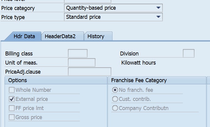
The price key used.

Execution

First we see DPC with Basic Category Determination of Current Periods via Meter Reading Results. The DPC category Read has been maintained as shown below in the Rate Category.

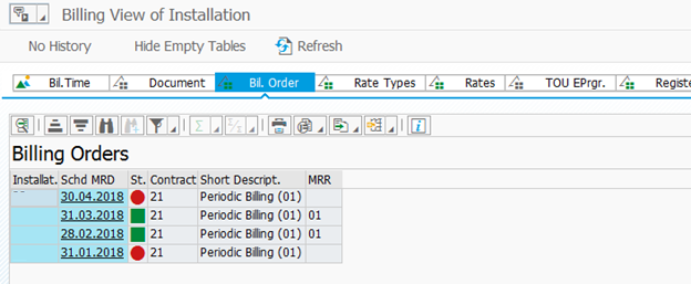
The Meter readings in the system is shown below which is not billed. The reading on 31.01.2018 and 30.04.2018 are actual readings while readings on 28.02.208 and 31.03.2018 are estimated readings.

Billing Document 07 is for reading on 31.01.2019 with actual Meter reading – 300. Similarly 08 document is for 28.02.2018(Estimated MR – 572 ) and 09 document is for 31.03.2018 (Estimated MR – 875) and 10 document is for actual reading on 30.04.2018 – 900 units. This triggers the back billing which we can see in the document. All these entries are present in EABL table. Also price change is taken into account.

When the current meter reading result is an estimate (category 1000 or 2000), both time slice generators (0000 and CONS) point to period to set up T with basic period category 4, which means variants QUANTI01, LUMSUM01, and DYNBI01 are each set up for the current periodic billing period. When an actual meter reading result is entered (category 3000 or 4000), time slice generator 0000 points to period to set up T, but CONS points to E, which has basic period category 3. In this case, variants LUMSUM01 and DYNBI01 are set up for the current periodic billing period. Variant QUANTI01 is set up for the period between the last and current actual meter reading results.Now the meter readings have been billed. The meter readings have not changed in EABL table.

The Billing Period Category are

These are the Period Categories

The start of each period to set up (except for the current periodic billing period) is taken from table ERCHP. This table is a supplemental table of the billing document, ERCH.

Now we see DPC with Basic Category Estimation of meter reading results in Billing. The DPC category Read has been maintained as shown below in the Rate Category.

The MRU shows the period in February and March with Estimated in Billing set to 01. For these two periods the readings will be estimated during Billing and no entry shall be made in EABL table. These two periods will have the status – Billable as shown in the below screenshot.

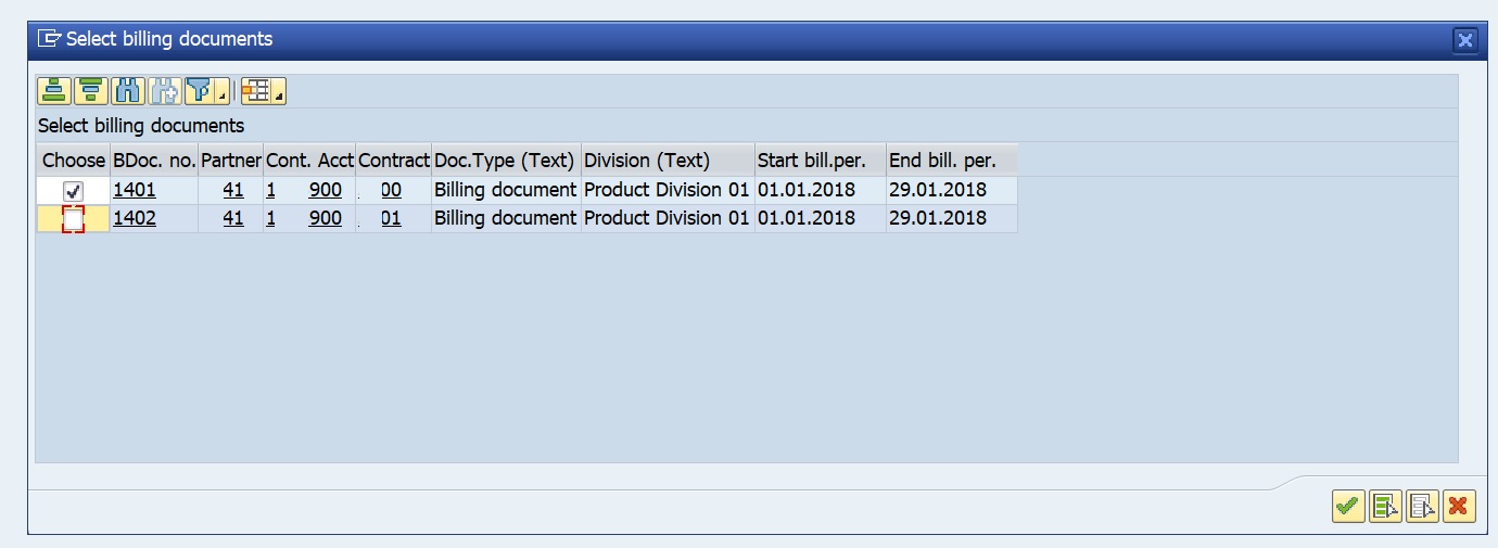
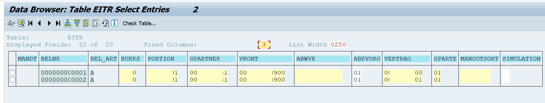
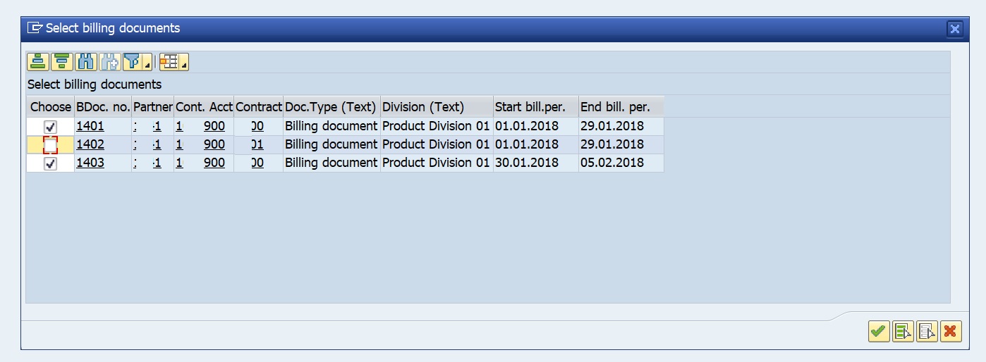
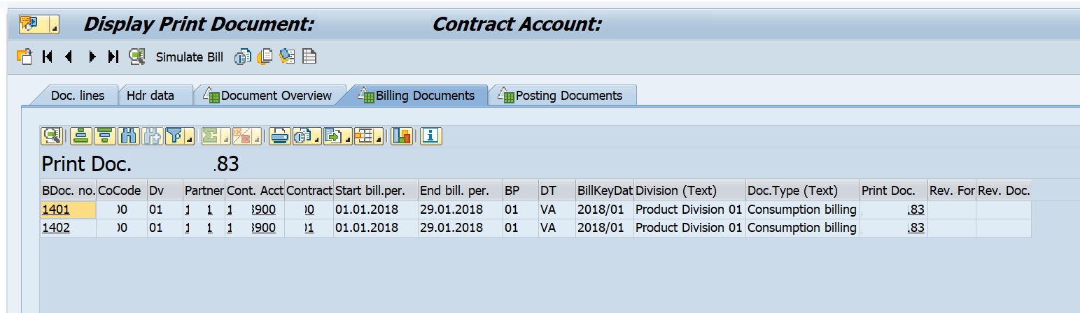
Billing Document 16 is for reading on 31.01.2019 with actual Meter reading – 300. Similarly 17 document is for 28.02.2018(Estimated MR in Billing ) and 18 document is for 31.03.2018 (Estimated MR in Billing) and 19 document is for actual reading on 30.04.2018 – 900 units. This triggers the back billing which we can see in the document. All actual readings are present in EABL table,Estimated readings in billing are not saved in EABL. Also price change is taken into account.

Now the meter readings have been billed. The meter readings have not changed in EABL table.

In the above Executions, I didn’t explicitly show how the Meter Reading can be changed for the back-billing periods.

Below we have a Billed Actual Read for 31.01.2018 and two Billed Estimated Read for 28.02.2018 and 31.03.2018.

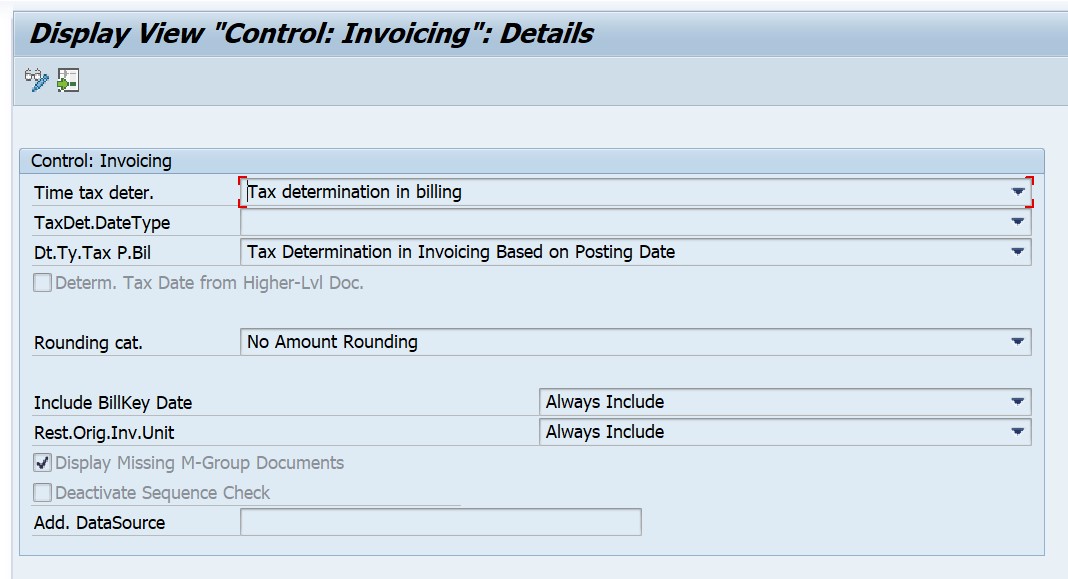
In configuration for Meter Reading Control Parameters we have the below setting.

If we check EL31 we can see even though we have Billing documents for the Estimated MR periods, the readings are still shown with status – Billable.

I can edit them as I have done below. Ignore the status 4 as I the reading had to be released from Implausibility. The point to note is that the readings have been changed for the period which has billing documents.  Also the Actual Read of 31.01.2018 is not editable and has the status 7 -Billed.

Now I have executed billing for April month and below we can see the details.

That’s it. Blog on Back billing coming soon.

Device Allocation

This blog post is about Device Allocations. The post on Billing Factor should have followed this one but somehow it got messed up. Anyways I was researching a scenario on Device Allocations specifically about the Device Allocation Type – Breaker Allocation and Gateway and the new Basic Device Category – Gateway.

About Device Allocation, it can be read online in the help site and in IUT 220. Written below are some of my notes which are just for further research/learning as has been my objective of these all blog posts. So kindly don’t mind the absence of screenshots here.

A Device Allocation would always contain a Controlling device and a Device that is been controlled.

Device Allocation Type describes the relationship between the installed devices.

The Controlling device and the Controlled device must be installed. They can be in installed in different installations.

The Controlled and Controlling devices must have the same division.

Depending on the Allocation type, both the devices must have certain attributes such as Basic Device Category.

Each device allocation has one allocation type.

There are 8 device Allocation Types predefined by SAP as shown earlier.

Each device allocation type has an attribute name. Attribute value is for information only. It is relevant for billing only for pressure regulator allocation (03) and transformer allocation (02).

In customizing the controlling device must have the Basic Device Category defined in the Allocation type.

Device allocation defined by the customer cannot be relevant to billing because the billing program only has access to the types of Device Allocation provided by SAP. (Check SAPLEG72 Include LEG72F10 – the logic for predefined allocation type is written here.)

The tables which matter in Device Allocation are

• EZUA – Device Allocation customizing table
• EZUG – Device Allocations for Register (Non – Metering Devices)
• EZUZ – Device Allocations for Register (Metering Devices)

Kindly note that the Logical Device Number (LOGIKNR) and Logical Register Number (LOGIKZW) play a huge part in the logic. Same does the function module ISU_METER_IDENTIFY (Determine a device uniquely based on Serial number).

For new Device Allocation type – Breaker Allocation and executed at Device Level, not register level, there is new logic written. The Controlling Device (Breaker) here should have the following characteristics

1. Controlling Device should be AMI.
2. AMCG (Advanced meter capability group) and AMSDG (advanced metering system determination group) should be maintained.
3. Controlling Device must have remote disconnection and reconnection capabilities.
4. As default, the Breaker can control only one device per time slice.

For a Controlled Device the following characteristics

1. Controlled Device should be a Meter.
2. The Controlled Device should have no remote disconnection and reconnection capabilities.
3. The Controlled Device should not be controlled by another Breaker in the same time slice.

For the Device Allocation Type – Gateway there’s no explicit code maintained which is surprising.

The function module which does the Billing Factor calculation is ISU_BILLING_FACTOR_DETERMINE and for Pressure regulator its ISU_PRESSURE_CHECK which reads table TE341.

For the Device Allocation Type – Gateway there’s no explicit code maintained which was surprising but it seems to have been handled in the web services.

A little bit on Gateways first – Gateways are to facilitate the automatic metered data entry in an intelligent metering system. Gateways are the medium between the meter technology and the energy data management system used by the utilities. The data can be stored for a specific time in the Gateway which works across divisions. This basic device category can be used to:

• Allocate smart meters from various divisions to a Gateway at device level. The Gateway acts as the controlling device here.
• Combine Gateways with other basic device categories, such as Other or Rate Switching Devices (ARCR – Audio frequency Ripple Control Receiver/Clock).

From a technical point of view, Gateways works like the basic device category Other but have their own combination and allocation settings.
Assignments are linked on device level only.
The Gateway functionality is activated with Business Function ISU_DM_1.
Any custom fields required for Gateway (or in general) can be done in Device Category (BAdI ISU_DM_DEVCAT) and in Devices (BAdI ISU_DM_DEVICE).

The webservice UtilitiesDeviceERPSmartMeterRelationshipNotification is triggered with the RoleCode “5” for Gateway allocations.

Allocation Type 08 is mapped to Role Code 5:

That’s it. Enjoy 😊

Billing Factor

This post is about Billing Factor. Lots of posts and Q&A can be found on the same if searched zealously. Here I am just commenting on how the SAP system is working to calculate the Billing Factor. This is as per standard behavior with no enhancements.

Billing Factor is the quotient calculated from the PT/CT ratio and Transformation Ratio of a meter attached with a transformer. The quotient is multiplied by the recorded consumption/demand, to determine the actual consumption/demand for billing.

The standard Function Module which calculates the Billing Factor is ISU_BILLING_FACTOR_DETERMINE.

The Billing factor is Transformer Factor divided by the Transformation Ratio.

The Transformation Ratio is a conversion factor. It is specific for a register which is allocated to the transformer. The Transformation Ratio is captured (if maintained) from the Register or Device or Device Category in that order. So, if the ratio is maintained in the register it is considered (highest priority). But if the Transformation Ratio is specified by maintaining the primary/Secondary voltage/current then that overwrites all ratios maintained anywhere mentioned above. Transformation Ratio is only maintainable for semi direct or indirect measuring type (maintained in Device Category)

The Function Module is drafted into 3 parts:
1. The Transformer Factor is fetched from the Controlling device (here Transformer)
2. The Transformation Ratio is fetched from the relevant object (search starts from the Controlled device) which has maintained it. Default Transformation Ratio is 1 (field name is ueberver).
3. The Billing Factor (field name is abrfakt) is determined for each register depending on the register Transformation Ratio and the factor of the Transformer allocated to it.

The below details are maintained in the Winding Group of the Transformer.

With the above details and the formula highlighted below the Transformer Factor comes to 40 (200/5) for the period.

Now the Transformation Ratio is fetched as per the hierarchy mentioned earlier if it’s not already calculated.

Now below code snipped shows how the Billing Factor is calculated. If the Transformer Ratio is maintained the IF part(line 492) is executed else the ELSE part(498) is executed.

The entire logic runs in loop depending on the registers as the Billing Factor is register dependent and time dependent.
Now the Billing Factor calculated by the system is 40. As we had maintained BILLFACALC parmater in customizing the calculated Billing Factor cannot overwrite any value we had given. It would give a message as shown below.

The customizing is shown below.

A brief recap – The Transformation Ratio can be maintained at Register level

or at the Device Level

or at the Device Category Level.

The Transformation Ratio can be calculated if the primary/Secondary voltage/current is maintained and this overwrites all ratios maintained anywhere mentioned above.

That’s it. Thanks, 😊

Convergent Invoicing: Billing Plan

This post is about Billing Plan(object) in Convergent Invoicing. As per SAP help by Using Billing Plans in Convergent Invoicing, the customer can define when and how frequently they receives an invoice and for what amount. In Utilities perspective, it almost like how Budget Billing works.

Billing Plan is assigned to a Contract or a Contract Account. The Billing Plan divides itself up into Plan Items and Billable Items. The Plan Items contain the rules and information for creating/generating Billable Items with specific amounts and for a predefined date. We can specify individual dates and amounts for the creation of Billable Items or define a Billing Cycle with a fixed amount for the creation of recurring Billable Items. These Billable Items are then invoiced.

The following scenarios are supported:

• Request/Refund of specific amounts at specified points of time
• Request of basic charges
• Payment Plans
• Discount Plans

The Processing for the above scenarios is done thorough at the level of Individual Billing Plan Items or the Billing Plan Item Types assigned to them.
Billing Plans can be processed periodically in a request run which determines the requested Billing Plan Items for the specified date and last request date and creates the relevant Billable Items.
To configure we need to configure some objects like Billing Plan Type – which controls the processing during Billing Plan item request together with the Billing Plan Item type, Billing Plan Category.
We need to configure the Offsetting Category – which controls the offsetting in Invoicing. The Interface Component needs to be activated for the Billing Class.

For the demo, I have configured a One-off Billing Plan and One Recurring Billing Plan. Not showing any configuration steps as its pretty basic with proper alignment of the Item type and Category with Billing Subprocess, Billable Item Type and Billable Class.

One-Off Billing Plan

Here, I am creating a Billing Plan for a One-Off Charge of 25 EUR for a Contract Account with unlimited Validity. By One Off charge, I mean it’s like an Incentive for the first subscription of an Offer.

The section highlighted would need to be filled manually. This process can be automated by executing program enhancements.

Below I have filled in the details as shown below. But I have limited the amount here (25 EUR) with Recurring Billing Plan Item checkbox unchecked.

So, when the Billing Plan is released and requested, this would create a One-Off charge Billable Item which can be Billed and Invoiced once requested.

Recurring Billing Plan

Here, I am creating a Billing Plan for a Recurring Charge of 100 EUR for a Contract Account with unlimited Validity for a Monthly Billing Cycle. By Recurring charge, I mean it’s like a Recurring Monthly Incentive for the subscription of an Offer. Below we can see that the Recurring Billing Plan checkbox is checked.

Now we Release the Billing Plan as shown below.

Once the Billing Plan is released, it looks like below with the Billing Cycle and the amount shown. Before being requested the value can still be changed, Once the Billing Plan is requested then any change would need reversal.

Transaction to create Billing Plan is FKKBIX_BILLPLAN. As shown below we can generate a request for Billing Plan Items.

The Billable Item is generated as shown below. The source transaction be default is BIP.

The billable Item can be Billed and Invoiced as shown below. The Reference Object would be BILLPLAN as shown below. The Invoice document shows the Billable Items considered.

That’s it.  😊

Joint Invoicing

This post is about the standard Joint Invoicing functionality provided. Would be more technical than functional as there’s not much scope of configuration here. Also, I would be touching on the technical aspects but deep dive into the logic is not there. This post would in a way be a guide on where to look if facing any issues or any enhancements for Joint Invoicing.

As per the definition in help.sap “Joint Invoicing is to ensure that IDocs and bills contain the same data during bill creation, it is technically not possible for multiple billing documents to be included together in one invoicing unit.”

This in a way summarizes what Joint Invoicing is supposed to achieve. As standard we have the following three options which are pretty simple to understand.
1 – Contracts must be invoiced together
2 – Contracts may be invoiced together
3 – Contracts must not be invoiced together

We have the Joint Invoicing field to be filled while executing the Move in and later replicated to the Contract. The customizing influencing the Joint Invoicing is present at Invoicing -> Basic Settings -> Define Basic Settings for Invoicing. The FQ Event is R403.

Let’s start with the demo then. I have two Contracts which have Joint Invoicing as 1. So, they must always be invoiced together with customizing not set and Event with standard functionality.

The FM which starts with the Invoicing is ISU_INV_SINGLE_PROCESSING. As I give the Contract Account for processing it picks up the Billing Document for both the Contracts as shown below. If I select one and execute it gives me the standard error for joint invoicing.

The Invoicing trigger is stored in table EITR – Temporary Selection Data for IS-U Invoicing shown below.

If I add another Bill for the first Contract (check the Billing period) we can see that I have an additional bill added in the selection while invoicing.

For forming the Invoicing unit, all the Billing documents relevant to Billable Contracts are picked up based on the billing document having the highest End Billing period date(p). So all Billing document whose End Billing period is less than p are selected. Once this is done its checked if each Contract has a billing document in the Invoicing Unit. If present then all green else we get the usual error message. In the above screenshot as I had only selected Billing documents for a single contract,it resulted in error.This logic is inside the Include LE21AF10 form CHECKUNIT_BILLING. This is called inside FM ISU_INV_UNIT_CHECK_BUILD.

Now I selected one document for each contract as shown below. If I select the billing document of a later period, the selection is terminated as prior period Bill in un-invoiced.

Now if I select the Billing Documents for each Contract leaving the latest one generated (1403) and execute Invoicing, I can see the Invoicing Document generated as shown below.

Now let’s check the customizing which is included in the code of FM ISU_INV_UNIT_CHECK_BUILD. The fields Include Bill Key Date, Restore Original Invoicing Unit and display Missing Documents play an role in the Joint Invoicing Process.

If the Bill Key Date is ‘Always Include’ then the Billing month like 2018/01 is also checked and Billing Document for the relevant period are grouped in the Invoicing unit. In out case , we have 3 Billing Document ,with the latest one with a different key date, so it shall be grouped in another Invoicing unit provided the joint Invoicing conditions also fulfill.

The event R403 which calls FM ISU_SAMPLE_R403 helps to modify the Invoicing unit formed by standard code.

Below we can see the code checks for missing document mentioned in the configuration.

Below we can see the code checks for original Invoicing unit mentioned in the configuration.

Below we can see the code checks for Bill key Date mentioned in the configuration.

Here, I had selected all the billing document with the configuration active for key date, as we can see it has taken the billing document for each contract with the same period. And left the latest billing document out.

External Price

Prices help to evaluate the Consumption or Demand in the system. We can define External Prices in the system where the prices are not maintained in the SAP system but passed by any other 3^rd party system. The logic for maintain prices then reside in the 3^rd party system with only the header details maintained in SAP.

In the header data of the Price we maintain the indicator for External Price as shown below.

The standard Enhancement object is EBIS0001 – ISU User exit for External Prices (EBL) with the Function Module – EXIT_SAPLEA91_001.

For all prices table EPREIH – History table for all prices is filled. For external prices this table would not have any entry. The Function Module which reads the prices during the Billing execution is ISU_PRICE_READ. In here based on External Price check, it executes the Exit and fetches the price details (takes into account the Price key and period) in EPREIH structure for processing.

The inputs required for the FM is Price Category, Pricing Level, From Date, To Date, Currency, Price Header and Key Date. For successful calculation the Y_OK_EXTERN flag should set to X.

The output should be in EPREIH structure. All the logic to decide on the Time Category or rounding or Price Blocks etc. would be done in the 3^rd party system with the final price passed back to SAP.

Scenario: I have to define a Fixed Term Contract where the price for the product (Electricity) wouldn’t change. Now the Prices are bound to change and same would be reflected for Non Fixed Term Contracts. Defining separate Price keys for Fixed/Non Fixed is not permissible as it would be unmanageable. So, I defined a unique External Price for Fixed Term contract which would refer (in code) to a custom table which have all the combinations and prices which the Fixed Term Contract should be billed for. Once the Fixed Term contract has reached an end , the Price key would be updated to the regular Price key and the entry in the custom table would be archived.

Convergent Invoicing: Invoicing of SD Billing Docs

This post is a continuation of the Convergent Invoicing posts(here). We can invoice SD billing documents in Convergent Invoicing. Other External documents can also be invoiced in Convergent Invoicing, provided proper customization is maintained.

In this post the focus is on Invoicing on SD Billing documents in Convergent Invoicing processes and not SD Billing documents functionalities/processes.

Using the invoicing function INV_VBRK_DOC (Invoice SD Billing Documents), we can process documents that are created in Sales and Distribution (SD) and then processed in Convergent Invoicing. The objects involved here are source documents to be invoiced of the source document category SD Billing Document (VBRK). If the source document category SD Documents (VBRK) is set by the Main Selection indicator, then an SD billing document can trigger Invoicing of the related contract account.

When an SD billing document is invoiced, the system adds the billing document to an invoicing unit and generates an invoicing document for each invoicing unit. In the invoicing document, the SD items are designated with invoicing item type 0VBRK_IT. These items are considered in the final invoice amount. The system manages an invoicing history and reversal history for the SD billing document.

An invoicing document item (DFKKINVDOC_I) is created for each business partner item. Along with the amount data, the invoicing document item adopts data such as the company code, account determination ID, and main and sub transaction.

The invoicing document item also receives a reference to the SD billing document from which it originates. This link is established by means of the fields SRCDOCCAT (Category of Source Document to Be Invoiced VBRK) and SRCDOCNO (Number of Source Document to Be Invoiced).

For SD billing we need to have some customization in place. I have configured a Sales Document Type in place.

This slideshow requires JavaScript.

Now I am creating a Sales Order for the new Order Type I created earlier. Transaction is VA01.

Gave the few mandatory details for the Sales Order and saved the same.

Now to create  SD Billing Document for the Sales Order created above. Transaction is VF01.

Now the SD Billing document must be released for Convergent Invoicing to process. This can be done in change mode. Transaction is VF02. Click on the button marked below, a success message would be shown in the status bar.

We can see in that the SD Billing document is now shown as an Invoicing Order to be processed in Convergent Invoicing.

But before that I am also creating some BIT items for the same Customer in Convergent Invoicing and executing the Billing also.

This slideshow requires JavaScript.

Now the Invoicing Order has the Billed BITs and the SD Billing Document as shown below.

When I execute Invoicing, we can see both the Invoicing Orders are populated and clubbed into Invoicing Units.

This slideshow requires JavaScript.

As the Invoicing function for SD was marked as Optional, I am now selecting it to be executed.

Now below are the Invoicing document details, which shows the details of the BITs from CI as well as details from the SD Billing Document.

This slideshow requires JavaScript.

Standard help document can be found here. That’s it.

TOU Exception & Response: Deep Dive

This is a short post on Time of Use Exception & Response. A continuation of an earlier post which can found here.

When we create TOU Exceptions based on Opt-In and Opt-out by the consumers, the Exceptions are created for the Contracts by default.

Say, we have 2 devices active for a Contract, then we would have 2 TOU Exceptions created, even if one of the device is not relevant for billing.

 

SAP provides Enhancement spots to change the way this works. The Enhancement spot is ISU_TOUEXCEPTRESP which provides BAdI for determining the level for Exception Creation (e.g. Exception creation at Contract level of Device or Register level) and how to handle the Exception creation.

This slideshow requires JavaScript.

SAP by default provides Exception Creation for Contract.  We can write code for Exception creation for Devices or Registers. That’s it. 😊